Documentation: Google Ads Reporting Script

This script, written in the Google Ads JavaScript API, is designed to create a comprehensive report of key PPC metrics for all of a company’s accounts and organize them into a Google Spreadsheet for the reference of the account owner(s).

Features:

  • Automatic report update: can be set to gather new data monthly, weekly, daily, or hourly depending on the needs of the team
  • Gathers key metrics: impressions, clicks, conversions, cost
  • Calculates other useful metrics: click-through rate, daily run rate, projected monthly spend
  • Allows the user to input budget for each account, providing more metrics: remaining budget, suggested daily run rate
  • Conditional formatting to provide an at-a-glance summary of which accounts need to spend more/less

Example output:

This script went through several versions. The initial prototype only outputted the last 30 days’ cost, impressions, clicks, and conversions data, and calculated the remaining budget. Additional features were added after discussions with the PPC team made it clear they would be helpful.

In addition, the code has gone through several alterations, independently of feature additions – mainly to streamline it. For example, in a previous version, metrics were collected daily and added to a sheet, then each column of that sheet was added together to produce a final result in a separate sheet. Now, data is collected as often as is desired, and there are no redundant sheets.

I wish I could post the code for you to use, but this project and its code are proprietary. However, if you’d like me to build something similar for you, feel free to contact me – I’d be happy to discuss!

Algorithm Design for Minimization of Time Complexity

This project requires a bit of background, for those who aren’t familiar with Google Ads. (For those who are, please skip down to the horizontal bar.)

When you search for something, some ads may show up at the top of the results page. Those ads were paid for by companies who had decided those ads were bringing in enough profit to be worth it.

Think about it in terms of four steps. 1, the company decides which keywords they want to bid on, and how much to bid on them. 2, the ads show up to users, and some percentage click through. 3, of those who click, some percentage actually convert (conversion defined however you decide – they may download a white paper, buy a product, or sign up for your email newsletter). 4, the company measures all aspects of this funnel and adjusts their keyword bids and/or ads accordingly.

This particular project involves automation of a specific portion of step 2. To try to maximize their ads’ conversion rates, marketers only want to serve their ads to people who have the highest chance of clicking, and ultimately, converting. A very important tool in the marketer’s arsenal for this goal is the negative.

Negatives, short for negative keywords, are keywords that tell the search engine that they should not display your ad if that keyword is part of the search query. For a quick example of why you might want to do this, consider that you’re running a bakery and you have two ads, one for cake recipes and one for carrot cake recipes. Now, obviously, you want only the cake recipe to show up when someone searches “cake recipe” or something similar, not when they search “carrot cake recipe” – you have a separate ad for that for a reason! So what you can do is make the word “carrot” a negative for your cake recipe ad.

This concept of negatives is useful for any circumstance where you don’t want your ad to show up – including because the keyword has a low conversion rate. And this is what this project is about.


This project involves taking a list of search terms and finding individual words which are always associated with a lack of conversions over an extended period of time and bringing them to the attention of the marketers running the ad campaigns so they can negative them. Therefore, it involves taking a table with a column of strings and a column of ints and isolating individual words (separated by spaces) which are associated with, and only with, int values of 0.

I considered a wide variety of possible algorithms in the course of working on this problem but ultimately wanted to find something which had a minimal time complexity and could run moderately quickly over tens of thousands of data points (six months or more worth of keywords and conversions).

I wanted to make sure I was looping through the dataset as few times as possible, so I would make sure to fetch the data, only store what I would absolutely need, and store it in a separate array so I didn’t have to deal with the hassle of deleting elements and having the machine shift everything else back, since I was liable to do a lot of deletions.

I will admit that this problem took me a long while to crack. I had too hard a time visualizing a massive dataset with so many different terms to think about doing any logically complicated data manipulations to it. So my first step was to simplify it to a little table, like this:

Strings | Ints
"a x" | 0
"a y" | 1
"b x" | 0
"b y" | 1

Abstracting away everything but the bare bones of the problem helped me finally realize what I succinctly described at the beginning of this essay, that I wanted to find all the elements with, and only with, an int (# of conversions) value of 0.

Once I removed that block, the ideas started pouring out. I went through about twenty different possibilities before settling on this basic concept:

  1. Fetch the data from an Excel spreadsheet to a Pandas DataFrame.
  2. Loop through the DataFrame, splicing each individual search term and splitting it into component words.
  3. Add each word associated with the number of conversions of the search term it’s a part of into another array, in alphabetical order.
  4. For each word in the resulting array, while the word is equal to the one in the next row after it, check if all conversion values are equivalent to each other and to 0.
  5. If they are, add the word to the final array; as soon as they’re not, skip to the next word and run that through step 4.

Now what’s left is to actually implement that. *exaggerated sigh*


What did you think of this post and this algorithm? Is it a good idea? Did I screw something up colossally? Please let me know in the comments below!

Thoughts on the Basics of Go

Disclaimer: I’ve been studying Go for two days. There are some neat things I learned about it, so I decided to document them, but if anything in this post is factually inaccurate, please let me know so I can correct it. Thanks!


Go is an object-oriented, statically-typed programming language created by Google in 2007, which makes it the only language I know that’s younger than me. (Python and JavaScript aren’t as young as you think they are, they were both created in the mid-90s. Yeah, I was surprised too.) Go seems to me like a weird lovechild of Java and JavaScript, but then again, I have heard it’s more like C, I just didn’t make that connection because I don’t know C.

That being said, if you already know both Java (or some other statically-typed OO language like C) and JavaScript (or some other dynamically-typed language like Python) most of the basics of Go aren’t going to seem odd to you. Go is statically typed, but it’s much smarter than Java in terms of inferring variable types, so the actual top-level programming feels somewhat like JavaScript or Python.

For some examples: Go has a main method that works just like Java, and one variable initialization style, var x int = 10, looks Java-esque. However, the idiomatic style for initializing variables looks somewhat like JavaScript: x := 10, since there’s no explicit type declaration. Overall, in Go, you type way less characters than you do in any other language I’ve used before. Look at the idiomatic initialization above. Or look at how you get a character from an array: arr[2], unlike Java, arr.charAt(2). The + operator is also overloaded to both addition and concatenation, like JavaScript, unlike the Java string.concat() method.

Now for the weird stuff that’s not like any other language I know – though it might be like some other language.

Go only has one loop, which happens to use the for keyword. Using different syntax patterns, it can operate like a for loop, a for-each loop, and a while loop, just to name a few. There’s also a range loop for k := range arr, and if another language I know uses them it’s definitely esoteric.

Go also does a weird thing with arrays. There are three standard types of array-like things: arrays, slices, and maps. Arrays pretty much work like Java: they have a set type and size and can’t be expanded. To fix the “arrays can’t be expanded but I wannaaaaa” problem, instead of going the Java route and making an array-style expandable object type which everyone then uses instead of standard arrays (ArrayList), Go has “slices”. These are segments of arrays which can be expanded when new elements are appended, until the length of the slice exceeds the length of the array, at which point the contents of the array are copied to a new array which is big enough to hold the appended elements. …I think. Maps are, fortunately, simpler. They’re sets of key-value pairs, where the keys and values can be of any single type. So you can map strings to ints, ints to ints, strings to strings, etc.

There are two things about Go which I find neither good nor bad, just very interesting. The first thing is that, among the variously-sized numeric types, there exist numeric types for complex numbers. This sparked a sudden desire in my mind to do something involving quantum physics with Go, although I have absolutely no idea what about quantum physics I would want to write a computer program for. The second thing is that Go does a lot of stuff in the Terminal, which makes me wonder how one goes about writing desktop applications in the language. (According to this article, it’s difficult.) I’m not a huge fan of web development stuff in general, and it’d be kind of annoying to have to make all my advanced Go projects web-based.

Besides slices, nothing about Go seems too awful or counterintuitive, so I’m optimistic about my future studies. As soon as I’ve got something a bit more complicated than Hello World, I’ll post projects and write-ups here. Please look forward to it!

What is a Feature Flag?

As a digital marketer, I wind up writing a decent number of articles for clients’ blogs. And as always happens when writing about a topic, I’ve learned a decent amount about these clients’ products. Our current biggest writing-focused client is Split, which is a B2B SaaS company selling feature flags as a service. But hold up, what on earth are feature flags? Well, I’m about to tell you.

A feature flag is a piece of conditional code that you wrap around any new feature, which links that feature to a dashboard. From this dashboard you can turn off the feature, release it to only a subset of your userbase, and generally manage all your features so you can see which ones are in use.

Now, how exactly is this useful? To start with, imagine a pre-existing codebase for a currently-working app. You don’t always start with this—one of the ways to implement continuous deployment is to start with a blank canvas—but this is usually how it works and is one of the most common feature flag use cases. Now, imagine a dev team working on a new feature to add to that app.

Without feature flags, this looks like a number of things, all of which are sub-optimal. You end up releasing only a few times a year because you need to do endless testing to make sure things aren’t broken before you push to production. You get crazy long-lived feature branches that take forever to merge back to trunk (“master” in Github terminology) and make a huge mess when they finally do. Or, worst, you accidentally break something but don’t realize until after you’ve already pushed to production, and you have to do a painful rollback to the previous version to fix the bugs, then re-release afterwards, and deal with the fallout from

With feature flags, the scenario looks much better. Instead of testing with your staff before pushing to production, just test in production on your real users—starting with just a select few of them, who have perhaps opted in to be guinea pigs. Instead of making branches which may or may not outlive their welcome and/or create a merge hell when you try to get them back to trunk, you can do everything straight in trunk. And if you break something anywhere in this process, you can just turn the feature off, no rollback required.

Beyond simply making development less of a headache overall, there are some specific things you can do with feature flags that are much harder otherwise. Some notable examples include continuous integration/delivery/deployment, canary releases and phased rollouts, and dark launches.

Continuous integration is the process of constantly and deliberately merging every code change to trunk (/master). Continuous delivery is constantly pushing each change to a production-like environment where there’s only one step of manual testing before it goes to end users. Continuous deployment is similar to continuous delivery, but without the manual testing: automated testing is the only step between the code deployment and the end users.

Canary releases and phased rollouts are similar in that they both involve releasing new features to only a subset of the userbase at first. With a canary release, the userbase subset is chosen and targeted to be test subjects, and they act like a canary in a coal mine, letting developers know whether the feature is safe to release to the broader public. With a phased rollout, you begin with a subset, which you then slowly ramp up until you’ve released to your entire userbase.

Dark launching is, literally, the process of launching a feature while keeping your users in the dark. Specifically, you use all the portions of your real infrastructure that would ordinarily be used in serving the feature, but you don’t actually show it to users. Feature flags can make this happen by letting you restrict access to only internal users, which lets the developers activate the feature in absence of a real code deployment.

There are a bunch more uses for feature flags – some of which are detailed on Split’s or FeatureFlags’s use cases pages, others can be found on Martin Fowler’s blog.

Priorities, Talks, and an Entirely-Un-Asked-For T-Shirt: Week 4 at Upgrow, Inc.

This week, as I promised I would do last week, I made a priority-ordered list of what needs to get done outside of work. Or, more properly, I decided on the One Thing that I’m going to do as much as possible for the next month, then laid out a rough timeline of the priorities for the rest of my apprenticeship.

In short, for the next month, I’m going to continue focusing on improving my Adulting On My Own skills, both in and outside the workplace. That means making sure I’m financially stable for the long haul, cultivating good relationships with my housemates as well as my coworkers, working on improving my marketing skills, and—this is the hard part—maintaining connections I made while I was staying at Reach.

I also got done a handful of other things which I didn’t plan to do in the last update but which are nonetheless very important. First off, I’ve started having weekly meetings on Friday evenings with Yitzchak, my Praxis pal who finally arrived in SF to work at the office in person about two weeks ago. This past meeting, we discussed humanism, religion, morality, and all other kinds of very fun deep topics.

That’s not all, and this last one surprised me too. After work on Tuesday, I was researching one of our clients in the hopes of understanding their industry better, and I ran across an industry talk the next day that the client was hosting at their office! I could not believe my luck and signed up for the talk right away, telling my advisors at Praxis that I couldn’t make the weekly Wednesday call. After work, I took a leisurely walk down to the office, had a nice dinner at a nearby burger place, and went to the talk. There were all kinds of cool people there, and the actual talk itself was about all sorts of cutting-edge time series database related stuff. I got to see a dashboard for a software that won’t exist until September! (No, I can’t show it to you, you perv. Wait till September like the rest of the public.)

After the talk, I chatted with a bunch of different people with the express intent of getting LinkedIn connections, because I’d eat a burrito with a fork before I’d walk away from a social event without making online connections. Turns out, one of the people I ended up talking to was the person on the client staff who hired our company in the first place! We had a super nice chat, discussed tech and marketing, and at the end she not only told me to help myself to the company-branded stickers they were handing out, she also grabbed me an entirely exclusive t-shirt and branded socks! I was literally so stoked. Nobody else got a t-shirt or socks! What did I do to deserve this privilege?? They’re really nice socks and I actually haven’t even taken them out of the packaging yet because they’re so awesome, although I did wear the t-shirt to work on Friday.

Anyway. It has officially been a month at this new job! Month 1 of 6 complete, and honestly it’s going pretty well. I’ve got a cheap and small but nice room in a group house with a signed lease and a security deposit, a relationship with my boss that’s moving in the direction of amicable, weekly discussions with a coworker that I’m becoming very good friends with, and some sweet company swag (and an open offer from my boss to maybe go to other client events to gather intel? what?). Next week, I’m going to work on doing a little bit more of all my stated goals, since I didn’t actually get around to making them in the first place till Wednesday and so I only had half a week to start implementing them. We’ll have to see how that goes; stay tuned!

PDP 5

Hey all! This update is coming in a little late, since I’ve been working through a bunch of interviews and projects for companies recently. After I get the definitive yes/no from those companies, I’ll see if I can post the projects here, but until then, here’s this week’s update.

This week, I learned in depth how to combat overfitting and faulty initialization, preprocess data, and a few state-of-the-art learning rate and gradient descent rules (including AdaGrad, RMSProp, and Adam). I also read some original ML research, and got started on doing my ML “Hello World”: the MNIST problem.

The section on overfitting was complete and explained the subject well, but the bit on initialization left me questioning a few things. For example, why do we use a sigmoid activation function if a lot of the possible values it can take (near 1, 0, and 0.5) are practically linear? Well, the answer, from the cutting-edge research, seems to be “we shouldn’t”. Xavier Glorot’s paper, Understanding the difficulty of training deep feedforward neural networks, explored a number of activation functions, and found that the sigmoid was one of the least useful, compared to the hyperbolic tangent and the softsign. To quote the paper, “We find that the logistic sigmoid activation is unsuited for deep networks with random initialization because of its mean value, which can drive especially the top hidden layer into saturation. […] We find that a new non-linearity that saturates less can often be beneficial.”

Within the course I’m using, section 41 deals with the state-of-the-art gradient descent rules. It’s exceedingly math-heavy, and took me a while to get through and understand. I found it helpful to copy down on paper all the relevant formulas, label the variables, and explain in short words what the different rules were for. Here’s part of a page of my notes.

I did teach myself enough calculus to understand the concepts of instantaneous rate of motion and partial derivative, which is all I’ve needed so far for ML. Here was the PDF I learned from, and which I will return to if I need to learn more.

The sections on preprocessing weren’t difficult to understand, but they did gloss over a decent amount of the detailed process, and I anticipate having a few minor difficulties when I start actually trying to preprocess real data. The part I don’t anticipate having any trouble with is deciding when to use binary versus one-hot encoding: they explain that bit relatively well. (Binary encoding involves sequential ordering of the categories, then converting those categories to binary and storing the 1 or 0 in an individual variable. One-hot encoding involves giving each individual item a 1 in a specific spot along a long list of length corresponding to the number of categories. You’d use binary encoding for large numbers of categories, but one-hot encoding for smaller numbers.)

The last thing I did was get started with MNIST. For anyone who hasn’t heard of it before, the MNIST data set is a large, preprocessed set of handwritten digits which can be categorically sorted by an ML algorithm into ten categories (the digits 0-9). I don’t have a lot to say about my process for doing this circa this week, but I’ll have an in-depth update on it next week when I finish it.

PDP 4

This week, I learned about deep learning and neural networks, and I wrote a handful of blog posts relating to concepts I learned last week.

The most poignant of these posts was Language: A Cluster Analysis of Reality. Taking inspiration from Eliezer Yudkowsky’s essay series A Human’s Guide To Words, and pieces of what I learned last week about cluster analyses, I created an abstract comparison between human language and cluster analyses done on n-dimensional reality-space.

Besides this, I started learning in depth about machine learning. I learned about the common loss functions, L2-norm and cross-entropy. I learned about the concept of deep neural nets: not just the theory, but the practice, all the way down to the math. I figured out what gradient descent is, and I’m getting started with TensorFlow. I’ll have more detail on all of this next week: there’s a lot I still don’t understand, and I don’t want to give a partially misinformed synopsis.

The most unfortunate part of this week was certainly that in order to fully understand deep neural networks, you need calculus, because a decent portion of the math relies on partial derivatives. I did statistics instead of calculus in high school, since I dramatically prefer probability theory to differential equations, so I don’t actually have all that much in the way of calculus, and there was an upper bound on how much of the math I actually got. I think that I’ll give myself a bit of remedial calculus in the next week.

The most fortunate part of this week was the discovery of how legitimately useful my favorite book is. Around four or five years ago, I read Rationality: From AI to Zombies. It’s written by a dude who’s big on AI, so obviously it contains rather a lot referencing that subject. When I first read it, I knew absolutely nothing about AI, so I just kind of skimmed over it, except to the extent that I was able to understand the fundamental theory by osmosis. However, I’ve been recently rereading Rationality for completely unrelated reasons, and the sections on AI are making a lot more sense to me now. The sections on AI are scattered through books 3, 4, and 5: The Machine in the Ghost, Mere Reality, and Mere Goodness.

And the most unexpected part of this week was that I had a pretty neat idea for a project, entirely unrelated to any of this other stuff I’ve been learning. I think I’ll program it in JavaScript over the next week, on top of this current project. It’s not complicated, so it shouldn’t get in the way of any of my higher-priority goals, but I had the idea because I would personally find it very useful. (Needless to say, I’ll be documenting that project on this blog, too.)

Language: A Cluster Analysis of Reality

Cluster analysis is the process of quantitatively grouping data in such a way that observations in the same group are more similar to each other than to those in other groups. This image should clear it up.

Whenever you do a cluster analysis, you do it on a specific set of variables: for example, I could cluster a set of customers against the two variables of satisfaction and brand loyalty. In that analysis, I might identify four clusters: (loyalty:high, satisfaction:low), (loyalty:low, satisfaction:low), (loyalty:high, satisfaction:high), and (loyalty:low, satisfaction:high). I might then label these four clusters to identify their characteristics for easy reference: “supporters”, “alienated”, “fans” and “roamers”, respectively.

What does that have to do with language?

Let’s take a word, “human”. If I define “human” as “featherless biped”, I’m effectively doing three things. One, I’m clustering an n-dimensional “reality-space”, which contains all the things in the universe graphed according to their properties, against the two variables ‘feathered’ and ‘bipedal’. Two, I’m pointing to the cluster of things which are (feathered:false, bipedal:true). Three, I’m labeling that cluster “human”.

This, the Aristotelian definition of “human”, isn’t very specific. It’s only clustering reality-space on two variables, so it ends up including some things that shouldn’t actually belong in the cluster, like apes and plucked chickens. Still, it’s good enough for most practical purposes, and assuming there aren’t any apes or plucked chickens around, it’ll help you to identify humans as separate from other things, like houses, vases, sandwiches, cats, colors, and mathematical theorems.

If we wanted to be more specific with our “human” definition, we could add a few more dimensions to our cluster analysis—add a few more attributes to our definition—and remove those outliers. For example, we might define “human” as “featherless bipedal mammals with red blood and 23 pairs of chromosomes, who reproduce sexually and use syntactical combinatorial language”. Now, we’re clustering reality-space against seven dimensions, instead of just two, and we get a more accurate analysis.

Despite this, we really can’t create a complete list of all the things that most real categories have in common. Our generalizations are leaky in some way, around the edges: our analyses aren’t perfect. (This is absolutely the case with every other cluster analysis, too.) There are always observations at the edges that might be in any number of clusters. Take a look at the graph above in this post. Those blue points at the top left edge, should they really be blue, or red or green instead? Are there really three clusters, or would it be more useful to say there are two, or four, or seven?

We make these decisions when we define words, too. Deciding which cluster to place an observation happens all the time with colors: is it red or orange, blue or green? Splitting one cluster into many happens when we need to split a word in order to convey more specific meaning: for example, “person” trisects into “human”, “alien”, and “AI”. Maybe you could split the “person” cluster even further than that. On the other end, you combine two categories into one when sub-cluster distinctions don’t matter for a certain purpose. The base-level category “table” substitutes more specific terms like “dining table” and “kotatsu” when the specifics don’t matter.

You can do a cluster analysis objectively wrong. There is math, and if the math says you’re wrong, you’re wrong. If your WCSS is so high that you have a cluster that you can’t label more distinctly than “everything else”, or if it’s so low you’ve segregated your clusters beyond the point of usefulness, then you’ve done it wrong.

Many people think “you can define a word any way you like”, but this doesn’t make sense. Words are cluster analyses of reality-space, and if cluster analyses can be wrong, words can also be wrong.


This post is a summary of / is based on Eliezer Yudkowsky’s essay sequence, “A Human’s Guide to Words“.

PDP 3

This week, I went even further in depth into doing statistical analyses in Python. I learned how to do logistic regressions and cluster analyses using k-means. I got a refresher on linear algebra, then used it to learn about the NumPy data type “ndarray”.

Logistic regressions are a bit complicated. The course I used explains it in a kind of strange way, which probably didn’t help. Fortunately, my mom knows a decent amount about statistical analyses (she used to be a researcher), so she was able to clear things up for me.

You do a logistic regression on a binary dependent variable. It ends up looking like a stretched-out S, either forwards or backwards. Data points are graphed on one of two lines, either y=0 or y=1. The regression line basically demonstrates a probability: how likely is it that you’ll pass an exam, given a certain number of study hours? How likely is it that you’ll get admitted to a college, given a certain SAT score? Practically, we care most about the tipping point, 50% probability, or y=0.5, and what values fall above and below that tipping point.

This can be slightly confusing since regression lines (or curves, for nonlinear regressions) usually predict values, but since there are only two possible values for a binary variable, the logistic regression line predicts a probability that a certain value will occur.

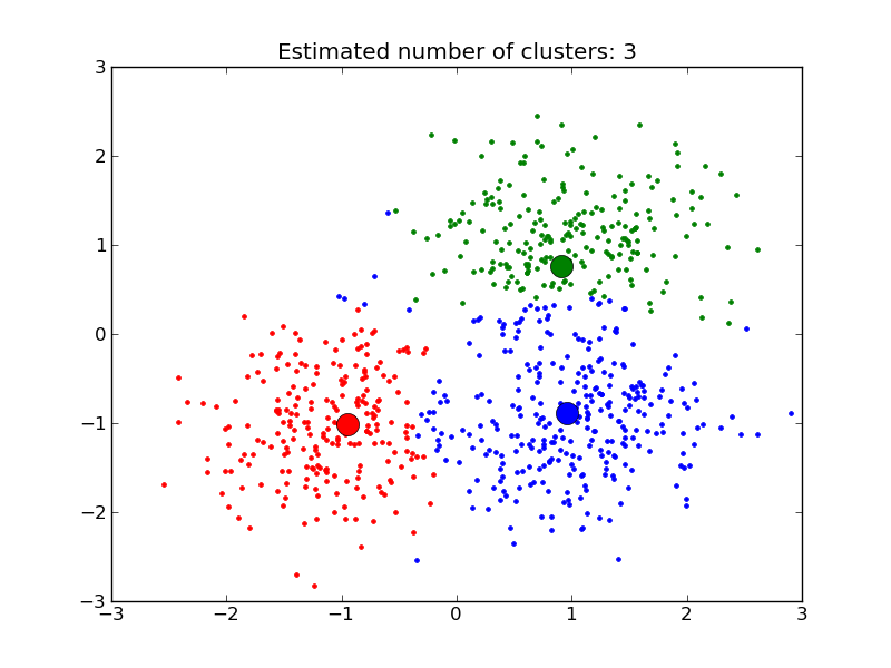
After I finished that, I moved on to K-means clustering, which is actually surprisingly easy. You randomly generate a number of centroids (generic term for the center of something, be it a line, polygon, cluster, etc.) corresponding to the number of clusters you want, and you assign points to centroids based on least Euclidean distance, move the centroids to the center of those new clusters, then assign the points to the centroids a second time.

Linear algebra is a little harder to understand, especially if your intuition isn’t visual like mine is. In essence, the basic object of linear algebra is a “tensor”, of which all other objects are types. A “scalar” is just an ordinary integer; a “vector” is a one-dimensional list of integers, and a “matrix” is a two-dimensional plane of integers, or a list of lists. These are tensors of type 0, 1, and 2, respectively. There are also tensors of type 3, which have no special name, as well as higher-order types.

I learned some basic linear algebra in school, but I figured it was a bit pointless. As it turns out though, linear algebra is incredibly useful for creating fast algorithms for multivariate algorithms, with many variables, many weights, and many constants. If you use standard integers (scalars) only, you’d need a formula like:
y1 + y2 + … + yk = (w1x1 + w2x2 + … + wkxk) + (b1 + b2 + … + bk).
But if you let all relevant variables be tensors, you can simplify that formula to:
y = wx + b

There are a handful of other awesome, useful ways to implement tensors. For example, image recognition. In order to represent an image as something the computer can do stuff with, we have to turn it into numbers. A type 3 tensor of the form 3xAxB, where AxB is the pixel dimension of the image in question, works perfectly. (Why use a third dimension of 3? Because images are commonly represented using the RGB, or Red/Green/Blue, color schema. In this, every color is represented with different values of R/G/B, between 0 and 255.)

Tensors, in the context of NumPy, which has a specific object type which is designed to handle them, are implemented using “ndarray”, or n-dimensional array. They’re not difficult to implement, and the notation is for once pretty straightforward. (It’s square brackets, similar to the mathematical notation.)

This should teach me to think of mathematical concepts as “pointless”. Computers think in math, so no matter how esoteric or silly the math seems, it’s part of how the computer thinks and I should probably learn it, for the same reasons I’ve devoted a lot of time to learning about all humans’ miscellaneous cognitive biases.

I’ve asked a handful of the statisticians I know if they wouldn’t mind providing some data for me to do some analyses of, since that would be a neat thing to do. But if I don’t do that, this coming week I’ll be learning in depth about AI, which my brain is already teeming with ideas for projects on. I’ve loved AI for a long time, and I’ve known how it works in theory for ages, but now I get to actually make one myself! I’m excited!

PDP 2

This week, I rehashed all the basics of Python. Since I haven’t studied it at all in ten years, this was a very useful refresher. (Basically, it seems to me that Python is essentially Java structure with something like JavaScript syntax. This is a huge oversimplification, but hey, it’s an extremely high-level language that I’m using it in an object-oriented way for this purpose. There are demonstrable similarities.)

The course I’m currently using doesn’t go over Python in any great detail, so if you’d like to supplement the Python they teach you, or you’d like to add to your knowledge of the language (since this course teaches only a very limited scope of Python), I highly recommend Learn Python The Hard Way. Python was my first programming language ever, and this was the course I used. It gives you a solid grasp of not just Python but how programming works in general.

In addition to the general Python refresher, I learned about all the libraries that I’ll need to use it to do data science: namely, NumPy, Pandas, SciPy, StatsModels API, MatPlotLib, Seaborn, and SciKitLearn. In combination, these libraries add methods that can import data from a variety of sources including Excel spreadsheets, conveniently calculate and tabulate relevant statistical data, do a variety of regressions and cluster analyses, and display elegant and understandable graphs.

This week, I learned how to do a simple linear regression (least squares). Next week, I’ll learn how to do multiple regressions and cluster analyses! And after that, the real fun begins with deep learning and AI. I’m looking forward to it!

In the future, expect me to start creating some little projects. I can’t do much with what I’ve learned this week, but by next week, I’ll absolutely have something at least moderately interesting, and I’ll absolutely do a nice write-up for it.